← Domain Convergence Research

Lattice Braiding Search

Spatially extended Fibonacci anyon braiding on 60-site chains — searching for genuine complexity

Overview

The braiding phase space search established that single-rule repetition on a finite Hilbert space cannot produce genuine complexity. This search extends to spatially extended systemsSystems where the dynamics happen across space, not just at a single point. Each location has its own state, and neighboring locations interact. Cellular automata and lattice models are spatially extended; a single oscillator is not.: 1D lattice chains where different braiding rules operate at different sites, producing emergent spatiotemporal patterns.

The motivation is physical: real topological systems involve many anyons distributed in space. Complexity might emerge from the interplay between local quantum dynamics (braiding) and spatial structure (the lattice pattern), even when each local operation is simple.

Read this as a deliberately-negative control. Both models use a product-state approximationEach site's quantum state is treated as independent — a 60×2 array rather than a 2⁶⁰ vector. Tractable, but it removes entanglement, the one quantum resource that could produce genuine complexity here. that removes entanglement, so we expect no genuine complexity going in. That makes the run useful as classifier calibrationRunning the method on a case whose true answer is known ("no genuine complexity") to measure how often the Wolfram-class classifier mislabels structured-but-simple behavior as complex — its false-positive rate.: the handful of "Class IV" hits below measure the false-positive rateThe fraction of cases flagged "Class IV / complex" when the ground truth is negative. Knowing this rate is what lets us discount apparent "complexity" found by the same classifier elsewhere. of the Wolfram-class classifier, not a discovery.

Method

Lattice model. A 1D chain of 60 Fibonacci anyons. Each adjacent pair has a local 2D fusion space. At each time step:

1. Apply braiding unitary U_A or U_B at each site according to a spatial pattern
2. Apply F-matrix coupling to propagate information between neighbors (coupling strength 0.3)

Rule selection. The top 50 rule pairs were selected from the single-rule search, ranked by commutator normA measure of how much two operations fail to commute — how different AB is from BA. Large commutator norm means the order of applying rules matters a lot, creating more potential for complex dynamics from rule interactions. (maximizing non-commutativity of the two rules).

Spatial patterns. 12 pattern types tested: uniform A, uniform B, alternating, period-3 (AAB), period-4 (ABBA), Fibonacci wordAn aperiodic binary sequence built by the substitution 0→01, 1→0 (producing 0, 01, 010, 01001, ...). Related to the golden ratio. Neither periodic nor random — it has a quasicrystalline structure with long-range order but no exact repetition., three random densities (30%, 50%, 70%), block (half/half), gradient, and Thue-MorseAn aperiodic binary sequence (0110100110010110...) built by repeatedly appending the complement. Overlap-free: no substring appears twice consecutively. Used as a test pattern for dynamics between order and chaos..

Two models:

• Linear model: Braiding rule at each site determined by the fixed spatial pattern. Product-state approximationTreating each site's quantum state as independent — a 60×2 array instead of a 2^60 vector. Computationally tractable but strips out entanglement, the very resource that makes quantum systems quantum. Also called mean-field approximation. (no entanglement between sites).
• Nonlinear model: Braiding rule at each site depends on the current state of its neighbor (if P(τ) > threshold, use rule B; otherwise rule A). This is a true CA with state-dependent update rules.

Total simulations: 1,570, split into 1,300 linear-model runs (50 rule pairs × 12 patterns × 2–3 configurations) and 270 nonlinear-model runs. The two models are tallied separately below, each against its own denominator.

Linear Model Results

Of the 1,300 linear-model runs:

Class	Count	Percentage	Description
I (fixed)	36	2.8%	Spatially uniform convergence
II (periodic)	1,149	88.4%	Spatiotemporal periodicity or standing waves
III (chaotic)	61	4.7%	Domain-wall dynamics and interference
IV (complex)	54	4.2%	Apparent spatiotemporal complexity (54/1,300)

Denominator note: 36 + 1,149 + 61 + 54 = 1,300 linear runs. The 270 nonlinear runs (0 Class IV) are tallied separately below, so the Class IV rate is 54/1,300 ≈ 4.2%.

Class IV distribution by spatial pattern

Pattern	Class IV count	Class IV rate	Notes
Period-4 (ABBA)	19	12.7%	Best performer by far
Fibonacci word	14	5.8%	Aperiodic structure helps
Random (30%)	4	8.0%	Low density + disorder
Period-3 (AAB)	8	5.3%	Moderate
Block (half/half)	5	2.1%	Single domain wall
Thue-Morse	4	2.7%	Substitution aperiodicity
Uniform A/B	0	0.0%	No spatial heterogeneity
Alternating	0	0.0%	Too regular
Random (50%, 70%)	0	0.0%	High density suppresses structure
Gradient	0	0.0%	Smooth variation not sufficient

The pattern is clear: intermediate structure wins. Period-4 ABBA (12.7% Class IV) and Fibonacci word (5.8%) both have the right balance of regularity and variation. Uniform patterns produce no complexity. Pure randomness at high density also fails.

Nonlinear Model Results

The nonlinear model applies state-dependent rule selection: if the left neighbor's P(τ) exceeds a threshold, use rule B; otherwise rule A. This creates a genuine CA where the update rule depends on the current state.

Class	Percentage	Description
II (periodic)	~88%	Threshold feedback creates fast lock-in
III (chaotic)	~12%	Period-doublingA route to chaos where oscillation period successively doubles: 1→2→4→8→... Governed by Feigenbaum's universal constants (δ ≈ 4.669). The same cascade appears in dripping faucets, heart tissue, and population models. to chaos
IV (complex)	0%	No complex intermediate (0/270)

The nonlinear model is worse for complexity. The threshold feedback overwhelms spatial pattern within approximately 20 timesteps, driving the system either to period-doubling cascades (Class III) or to stable oscillations (Class II). There is no complex intermediate regime.

Honest Assessment

The Fundamental Bottleneck

Paths Forward

Four approaches could break through the entanglement barrier.

1. Matrix Product StateA compact representation of quantum states that captures entanglement up to a tunable bond dimension χ. The sweet spot between full simulation (exponentially expensive) and product-state (no entanglement). Standard tool in condensed matter physics. (MPS) simulation. Represent the chain as an MPS with bond dimension chi. This captures entanglement up to chi correlations. Cost: O(N chi³) per step. For 60 sites at chi=64, this is feasible on modern hardware.¹ The question: does entanglement entropy grow with time (indicating genuine complexity) or saturate (indicating topological order without dynamics)?
2. Measurement-based dynamics. Intersperse braiding with projective measurements. This breaks unitarity and can create genuinely irreversible dynamics. The measurement collapses entanglement locally, but the braiding re-creates it. The interplay might support complex dynamics.
3. Dissipative coupling (Lindblad dynamics). Add controlled decoherence via a Lindblad master equationThe most general equation for open quantum system evolution that preserves probability and positivity. Adds controlled decoherence to unitary dynamics — modeling how a quantum system loses information to its environment. Breaks time-reversibility.. This models a topological system coupled to an environment. Dissipation breaks unitarity and can drive the system to non-equilibrium steady states with complex structure.
4. Smooth nonlinear feedback. Replace the binary threshold with a smooth function (e.g., tanh with adjustable steepness). The binary threshold is a singular limit that destroys intermediate behavior. A smooth feedback function might support a richer dynamical landscape.

Plots

Linear model: Class IV candidates

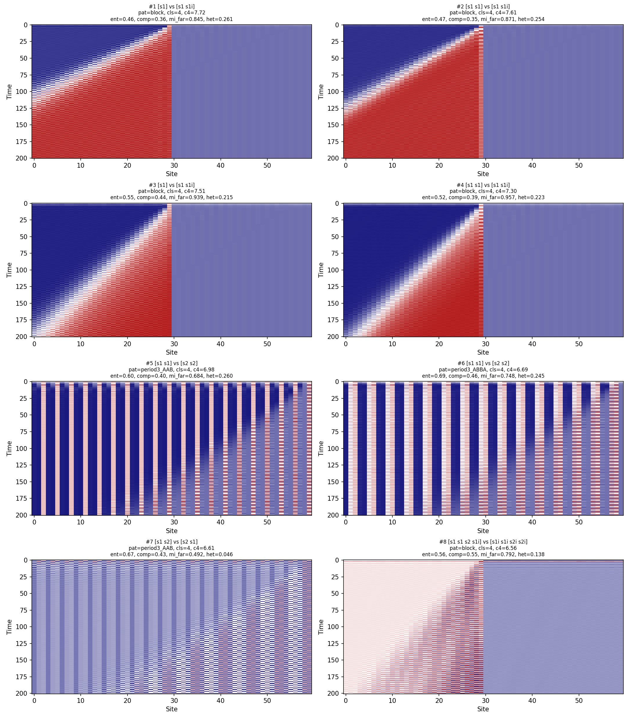
Spacetime diagrams for the top Class IV candidates in the linear lattice model. Horizontal axis: site position (60 sites). Vertical axis: time (200 steps). Color: P(τ) at each site. The patterns show domain-wall interference, not genuine complexity.

Linear model: Class IV by spatial pattern

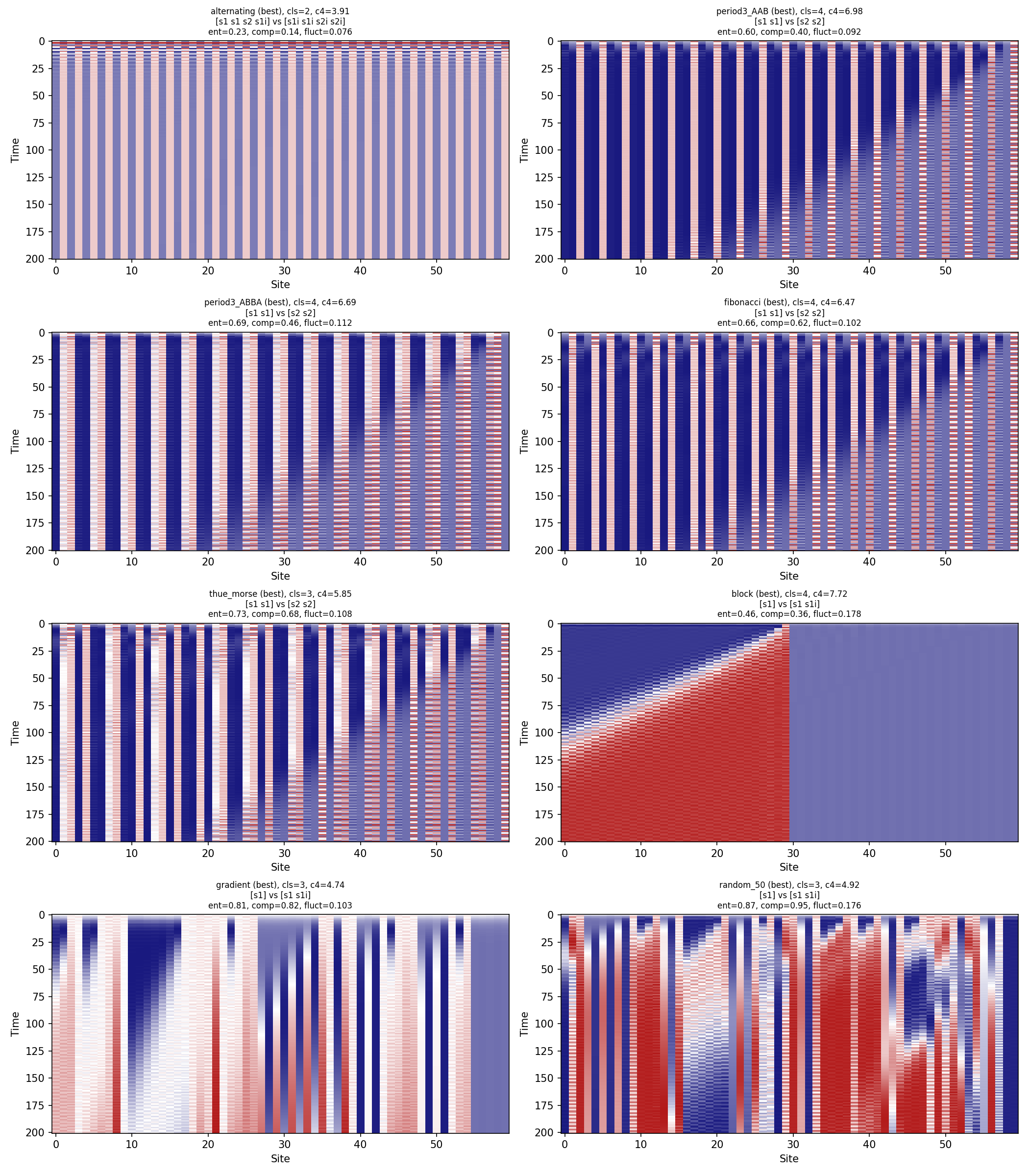
Class IV candidate distribution across spatial pattern types. Period-4 ABBA dominates at 12.7% Class IV rate. Fibonacci word is second at 5.8%. Uniform and alternating patterns produce zero Class IV.

Nonlinear model: candidate trajectories

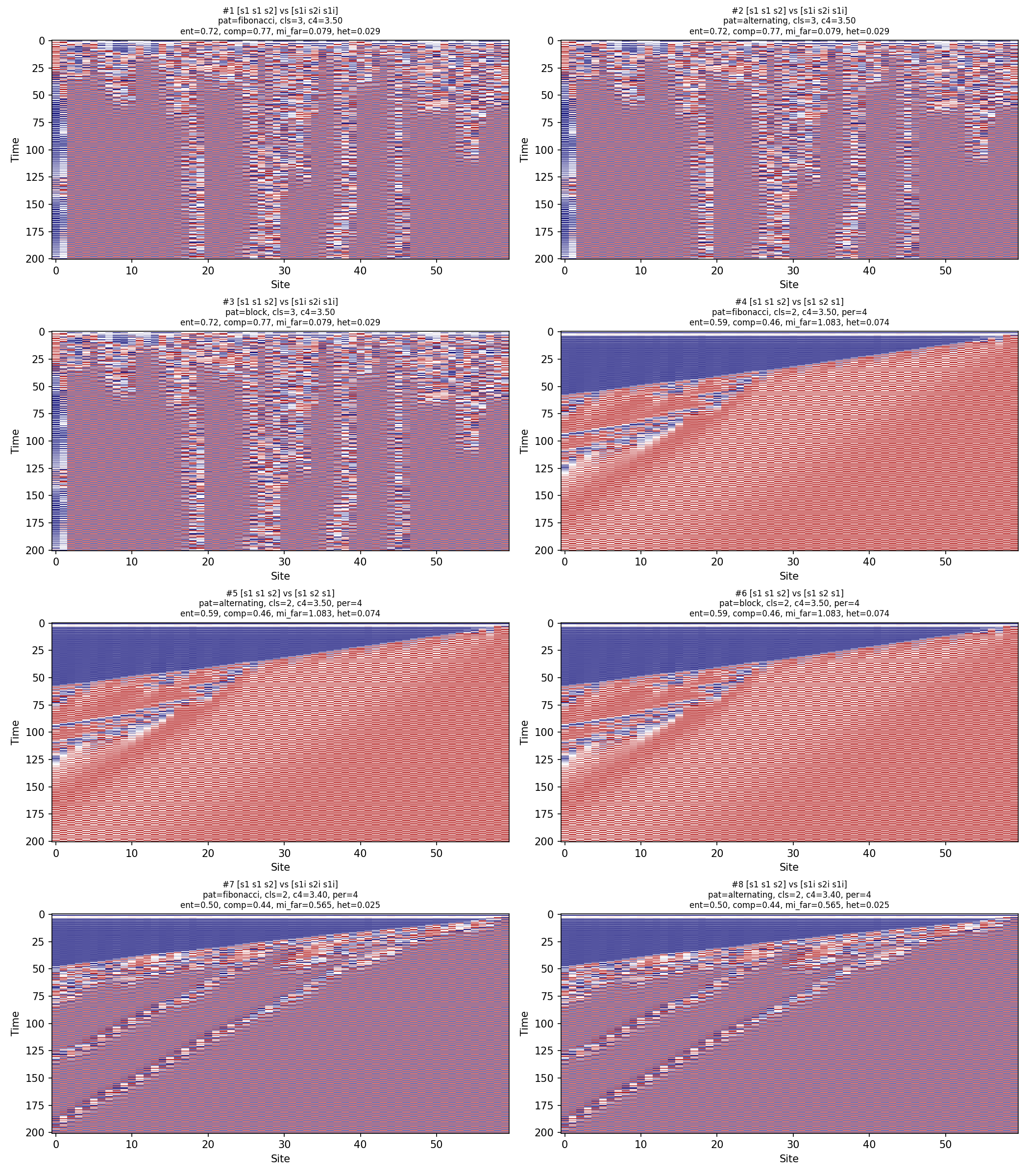
Nonlinear model (state-dependent rule selection). The threshold feedback drives the system to period-doubling cascades within ~20 timesteps. No complex intermediate regime.

Nonlinear model: by spatial pattern

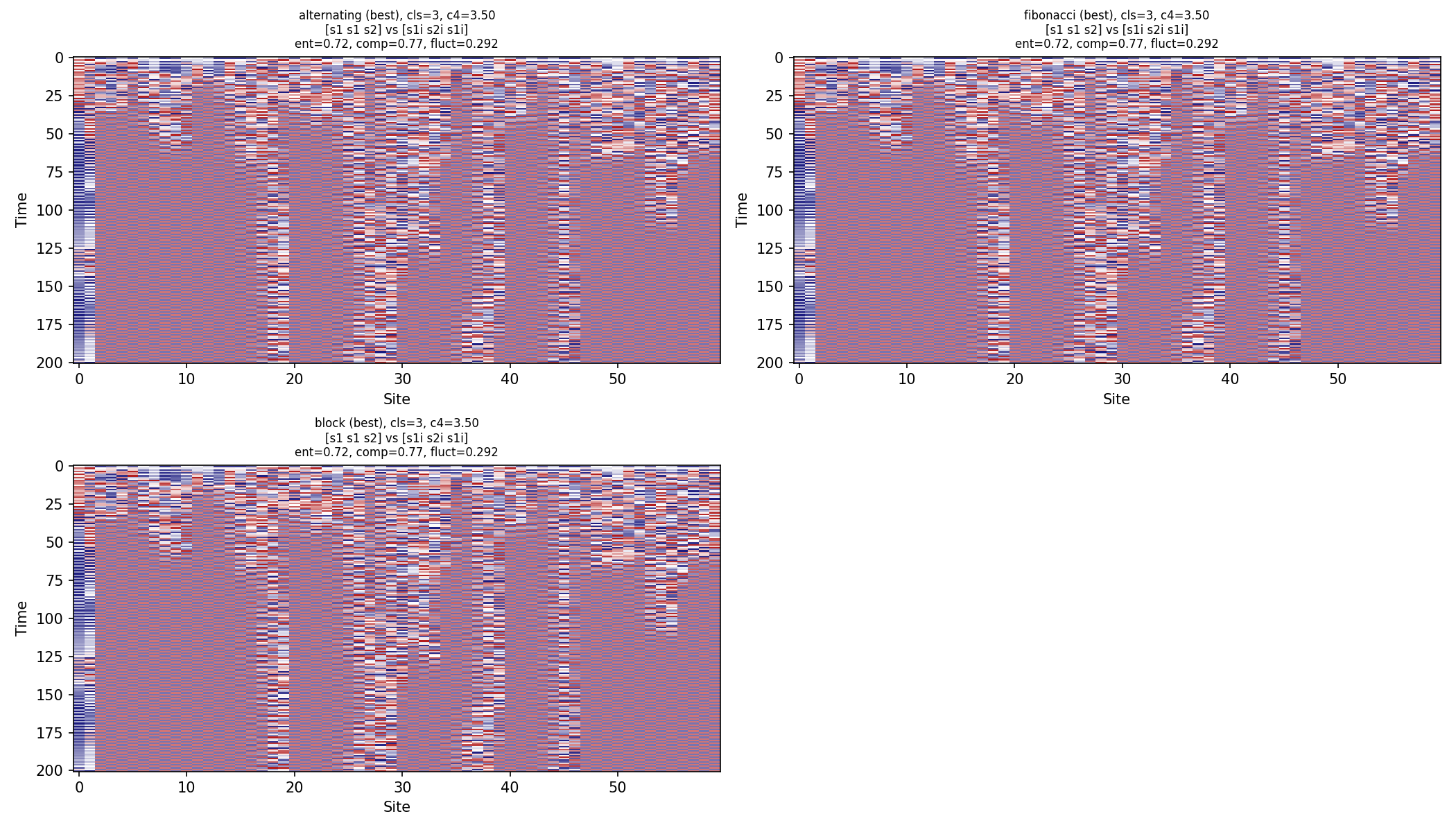
Nonlinear model results grouped by spatial pattern. The threshold feedback mechanism dominates over the spatial pattern: all patterns converge to similar periodic or chaotic behavior within 20 steps.